Page 440 - Python Data Science Handbook

The binary splitting makes this extremely efficient: in a well-constructed tree, each
question will cut the number of options by approximately half, very quickly narrow‐
ing the options even among a large number of classes. The trick, of course, comes in
deciding which questions to ask at each step. In machine learning implementations of
decision trees, the questions generally take the form of axis-aligned splits in the data;
that is, each node in the tree splits the data into two groups using a cutoff value
within one of the features. Let’s now take a look at an example.

Creating a decision tree
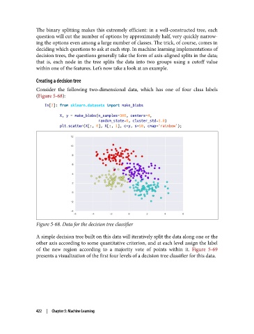
Consider the following two-dimensional data, which has one of four class labels
(Figure 5-68):

In[2]: from sklearn.datasets import make_blobs
X, y = make_blobs(n_samples=300, centers=4,
random_state=0, cluster_std=1.0)
plt.scatter(X[:, 0], X[:, 1], c=y, s=50, cmap='rainbow');

Figure 5-68. Data for the decision tree classifier

A simple decision tree built on this data will iteratively split the data along one or the
other axis according to some quantitative criterion, and at each level assign the label
of the new region according to a majority vote of points within it. Figure 5-69
presents a visualization of the first four levels of a decision tree classifier for this data.

422 | Chapter 5: Machine Learning