Page 451 - Python Data Science Handbook

A primary disadvantage of random forests is that the results are not easily interpreta‐
ble; that is, if you would like to draw conclusions about the meaning of the classifica‐
tion model, random forests may not be the best choice.
In Depth: Principal Component Analysis

Up until now, we have been looking in depth at supervised learning estimators: those
estimators that predict labels based on labeled training data. Here we begin looking at
several unsupervised estimators, which can highlight interesting aspects of the data
without reference to any known labels.
In this section, we explore what is perhaps one of the most broadly used of unsuper‐
vised algorithms, principal component analysis (PCA). PCA is fundamentally a
dimensionality reduction algorithm, but it can also be useful as a tool for visualiza‐
tion, for noise filtering, for feature extraction and engineering, and much more. After
a brief conceptual discussion of the PCA algorithm, we will see a couple examples of
these further applications. We begin with the standard imports:

In[1]: %matplotlib inline
import numpy as np
import matplotlib.pyplot as plt
import seaborn as sns; sns.set()

Introducing Principal Component Analysis
Principal component analysis is a fast and flexible unsupervised method for dimen‐
sionality reduction in data, which we saw briefly in “Introducing Scikit-Learn” on
page 343. Its behavior is easiest to visualize by looking at a two-dimensional dataset.
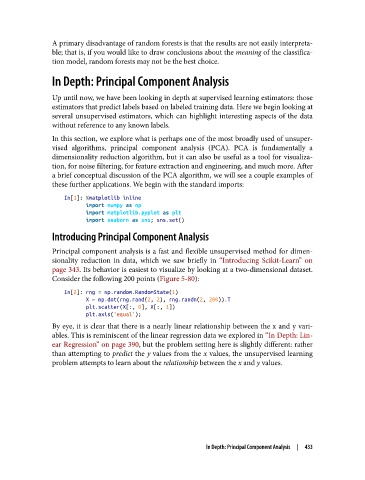
Consider the following 200 points (Figure 5-80):

In[2]: rng = np.random.RandomState(1)
X = np.dot(rng.rand(2, 2), rng.randn(2, 200)).T
plt.scatter(X[:, 0], X[:, 1])
plt.axis('equal');
By eye, it is clear that there is a nearly linear relationship between the x and y vari‐
ables. This is reminiscent of the linear regression data we explored in “In Depth: Lin‐
ear Regression” on page 390, but the problem setting here is slightly different: rather
than attempting to predict the y values from the x values, the unsupervised learning
problem attempts to learn about the relationship between the x and y values.

In Depth: Principal Component Analysis | 433