Page 452 - Python Data Science Handbook

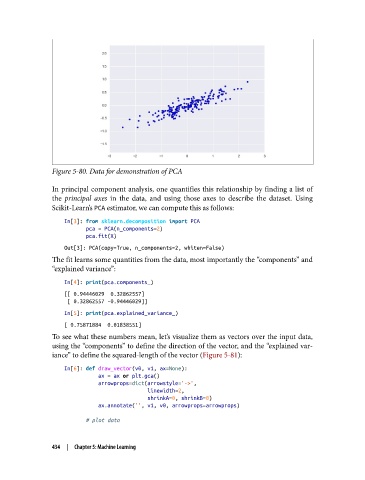
Figure 5-80. Data for demonstration of PCA

In principal component analysis, one quantifies this relationship by finding a list of
the principal axes in the data, and using those axes to describe the dataset. Using
Scikit-Learn’s PCA estimator, we can compute this as follows:

In[3]: from sklearn.decomposition import PCA
pca = PCA(n_components=2)
pca.fit(X)
Out[3]: PCA(copy=True, n_components=2, whiten=False)
The fit learns some quantities from the data, most importantly the “components” and
“explained variance”:

In[4]: print(pca.components_)
[[ 0.94446029 0.32862557]
[ 0.32862557 -0.94446029]]
In[5]: print(pca.explained_variance_)
[ 0.75871884 0.01838551]
To see what these numbers mean, let’s visualize them as vectors over the input data,
using the “components” to define the direction of the vector, and the “explained var‐
iance” to define the squared-length of the vector (Figure 5-81):

In[6]: def draw_vector(v0, v1, ax=None):
ax = ax or plt.gca()
arrowprops=dict(arrowstyle='->',
linewidth=2,
shrinkA=0, shrinkB=0)
ax.annotate('', v1, v0, arrowprops=arrowprops)

# plot data

434 | Chapter 5: Machine Learning