Page 454 - Python Data Science Handbook

This transformation from data axes to principal axes is as an a‘ne transformation,
which basically means it is composed of a translation, rotation, and uniform scaling.
While this algorithm to find principal components may seem like just a mathematical
curiosity, it turns out to have very far-reaching applications in the world of machine
learning and data exploration.

PCA as dimensionality reduction
Using PCA for dimensionality reduction involves zeroing out one or more of the
smallest principal components, resulting in a lower-dimensional projection of the
data that preserves the maximal data variance.
Here is an example of using PCA as a dimensionality reduction transform:

In[7]: pca = PCA(n_components=1)
pca.fit(X)
X_pca = pca.transform(X)
print("original shape: ", X.shape)
print("transformed shape:", X_pca.shape)
original shape: (200, 2)
transformed shape: (200, 1)
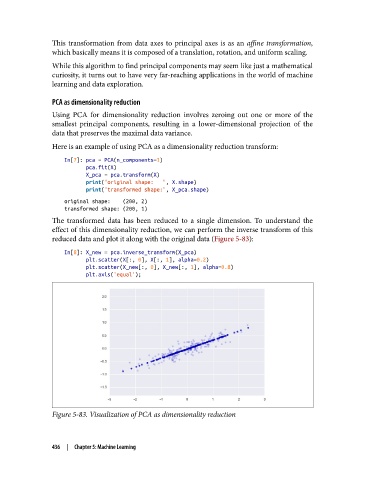
The transformed data has been reduced to a single dimension. To understand the
effect of this dimensionality reduction, we can perform the inverse transform of this
reduced data and plot it along with the original data (Figure 5-83):

In[8]: X_new = pca.inverse_transform(X_pca)
plt.scatter(X[:, 0], X[:, 1], alpha=0.2)
plt.scatter(X_new[:, 0], X_new[:, 1], alpha=0.8)
plt.axis('equal');

Figure 5-83. Visualization of PCA as dimensionality reduction

436 | Chapter 5: Machine Learning