Page 458 - Python Data Science Handbook

Choosing the number of components

A vital part of using PCA in practice is the ability to estimate how many components
are needed to describe the data. We can determine this by looking at the cumulative
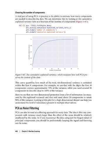
explained variance ratio as a function of the number of components (Figure 5-87):
In[12]: pca = PCA().fit(digits.data)
plt.plot(np.cumsum(pca.explained_variance_ratio_))
plt.xlabel('number of components')
plt.ylabel('cumulative explained variance');

Figure 5-87. The cumulative explained variance, which measures how well PCA pre‐
serves the content of the data

This curve quantifies how much of the total, 64-dimensional variance is contained
within the first N components. For example, we see that with the digits the first 10
components contain approximately 75% of the variance, while you need around 50
components to describe close to 100% of the variance.

Here we see that our two-dimensional projection loses a lot of information (as meas‐
ured by the explained variance) and that we’d need about 20 components to retain
90% of the variance. Looking at this plot for a high-dimensional dataset can help you
understand the level of redundancy present in multiple observations.

PCA as Noise Filtering

PCA can also be used as a filtering approach for noisy data. The idea is this: any com‐
ponents with variance much larger than the effect of the noise should be relatively
unaffected by the noise. So if you reconstruct the data using just the largest subset of
principal components, you should be preferentially keeping the signal and throwing
out the noise.

440 | Chapter 5: Machine Learning