Page 460 - Python Data Science Handbook

In[15]: pca = PCA(0.50).fit(noisy)
pca.n_components_
Out[15]: 12
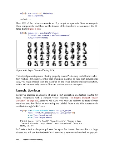
Here 50% of the variance amounts to 12 principal components. Now we compute
these components, and then use the inverse of the transform to reconstruct the fil‐
tered digits (Figure 5-90):

In[16]: components = pca.transform(noisy)
filtered = pca.inverse_transform(components)
plot_digits(filtered)

Figure 5-90. Digits “denoised” using PCA

This signal preserving/noise filtering property makes PCA a very useful feature selec‐
tion routine—for example, rather than training a classifier on very high-dimensional
data, you might instead train the classifier on the lower-dimensional representation,
which will automatically serve to filter out random noise in the inputs.
Example: Eigenfaces

Earlier we explored an example of using a PCA projection as a feature selector for
facial recognition with a support vector machine (“In-Depth: Support Vector
Machines” on page 405). Here we will take a look back and explore a bit more of what
went into that. Recall that we were using the Labeled Faces in the Wild dataset made
available through Scikit-Learn:
In[17]: from sklearn.datasets import fetch_lfw_people
faces = fetch_lfw_people(min_faces_per_person=60)
print(faces.target_names)
print(faces.images.shape)
['Ariel Sharon' 'Colin Powell' 'Donald Rumsfeld' 'George W Bush'
'Gerhard Schroeder' 'Hugo Chavez' 'Junichiro Koizumi' 'Tony Blair']
(1348, 62, 47)
Let’s take a look at the principal axes that span this dataset. Because this is a large
dataset, we will use RandomizedPCA—it contains a randomized method to approxi‐

442 | Chapter 5: Machine Learning