Page 461 - Python Data Science Handbook

mate the first N principal components much more quickly than the standard PCA esti‐
mator, and thus is very useful for high-dimensional data (here, a dimensionality of
nearly 3,000). We will take a look at the first 150 components:
In[18]: from sklearn.decomposition import RandomizedPCA
pca = RandomizedPCA(150)
pca.fit(faces.data)
Out[18]: RandomizedPCA(copy=True, iterated_power=3, n_components=150,
random_state=None, whiten=False)
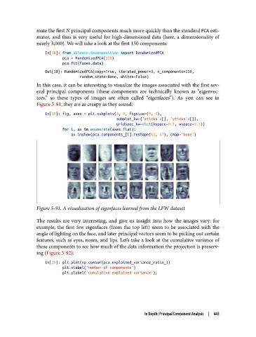
In this case, it can be interesting to visualize the images associated with the first sev‐
eral principal components (these components are technically known as “eigenvec‐
tors,” so these types of images are often called “eigenfaces”). As you can see in
Figure 5-91, they are as creepy as they sound:
In[19]: fig, axes = plt.subplots(3, 8, figsize=(9, 4),
subplot_kw={'xticks':[], 'yticks':[]},
gridspec_kw=dict(hspace=0.1, wspace=0.1))
for i, ax in enumerate(axes.flat):
ax.imshow(pca.components_[i].reshape(62, 47), cmap='bone')

Figure 5-91. A visualization of eigenfaces learned from the LFW dataset

The results are very interesting, and give us insight into how the images vary: for
example, the first few eigenfaces (from the top left) seem to be associated with the
angle of lighting on the face, and later principal vectors seem to be picking out certain
features, such as eyes, noses, and lips. Let’s take a look at the cumulative variance of
these components to see how much of the data information the projection is preserv‐
ing (Figure 5-92):

In[20]: plt.plot(np.cumsum(pca.explained_variance_ratio_))
plt.xlabel('number of components')
plt.ylabel('cumulative explained variance');

In Depth: Principal Component Analysis | 443