Page 226 - Python Data Science Handbook

With this in mind, let’s do a compound groupby and look at the hourly trend on
weekdays versus weekends. We’ll start by grouping by both a flag marking the week‐
end, and the time of day:
In[45]: weekend = np.where(data.index.weekday < 5, 'Weekday', 'Weekend')
by_time = data.groupby([weekend, data.index.time]).mean()
Now we’ll use some of the Matplotlib tools described in “Multiple Subplots” on page
262 to plot two panels side by side (Figure 3-17):

In[46]: import matplotlib.pyplot as plt
fig, ax = plt.subplots(1, 2, figsize=(14, 5))
by_time.ix['Weekday'].plot(ax=ax[0], title='Weekdays',
xticks=hourly_ticks, style=[':', '--', '-'])
by_time.ix['Weekend'].plot(ax=ax[1], title='Weekends',
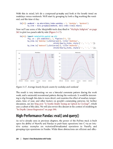
xticks=hourly_ticks, style=[':', '--', '-']);

Figure 3-17. Average hourly bicycle counts by weekday and weekend

The result is very interesting: we see a bimodal commute pattern during the work
week, and a unimodal recreational pattern during the weekends. It would be interest‐
ing to dig through this data in more detail, and examine the effect of weather, temper‐
ature, time of year, and other factors on people’s commuting patterns; for further
discussion, see my blog post “Is Seattle Really Seeing an Uptick In Cycling?”, which
uses a subset of this data. We will also revisit this dataset in the context of modeling in
“In Depth: Linear Regression” on page 390.

High-Performance Pandas: eval() and query()

As we’ve already seen in previous chapters, the power of the PyData stack is built
upon the ability of NumPy and Pandas to push basic operations into C via an intu‐
itive syntax: examples are vectorized/broadcasted operations in NumPy, and
grouping-type operations in Pandas. While these abstractions are efficient and effec‐

208 | Chapter 3: Data Manipulation with Pandas