Page 266 - Python Data Science Handbook

plt.hexbin: Hexagonal binnings

The two-dimensional histogram creates a tessellation of squares across the axes.
Another natural shape for such a tessellation is the regular hexagon. For this purpose,
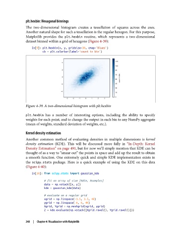
Matplotlib provides the plt.hexbin routine, which represents a two-dimensional
dataset binned within a grid of hexagons (Figure 4-39):

In[9]: plt.hexbin(x, y, gridsize=30, cmap='Blues')
cb = plt.colorbar(label='count in bin')

Figure 4-39. A two-dimensional histogram with plt.hexbin

plt.hexbin has a number of interesting options, including the ability to specify
weights for each point, and to change the output in each bin to any NumPy aggregate
(mean of weights, standard deviation of weights, etc.).

Kernel density estimation

Another common method of evaluating densities in multiple dimensions is kernel
density estimation (KDE). This will be discussed more fully in “In-Depth: Kernel
Density Estimation” on page 491, but for now we’ll simply mention that KDE can be
thought of as a way to “smear out” the points in space and add up the result to obtain
a smooth function. One extremely quick and simple KDE implementation exists in
the scipy.stats package. Here is a quick example of using the KDE on this data
(Figure 4-40):

In[10]: from scipy.stats import gaussian_kde
# fit an array of size [Ndim, Nsamples]
data = np.vstack([x, y])
kde = gaussian_kde(data)
# evaluate on a regular grid
xgrid = np.linspace(-3.5, 3.5, 40)
ygrid = np.linspace(-6, 6, 40)
Xgrid, Ygrid = np.meshgrid(xgrid, ygrid)
Z = kde.evaluate(np.vstack([Xgrid.ravel(), Ygrid.ravel()]))

248 | Chapter 4: Visualization with Matplotlib