Page 285 - Python Data Science Handbook

itself; it is simply a convenient interface that is recognized by the plt.subplot()
command. For example, a gridspec for a grid of two rows and three columns with
some specified width and height space looks like this:
In[8]: grid = plt.GridSpec(2, 3, wspace=0.4, hspace=0.3)
From this we can specify subplot locations and extents using the familiar Python slic‐
ing syntax (Figure 4-65):
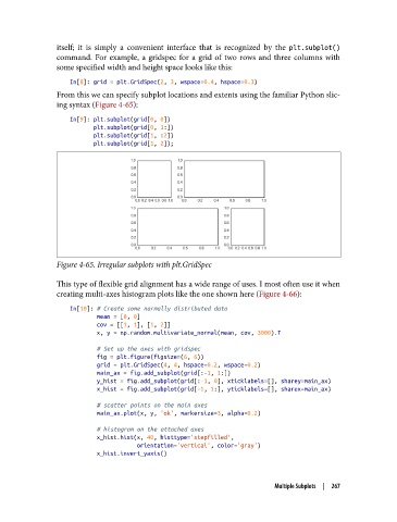
In[9]: plt.subplot(grid[0, 0])
plt.subplot(grid[0, 1:])
plt.subplot(grid[1, :2])
plt.subplot(grid[1, 2]);

Figure 4-65. Irregular subplots with plt.GridSpec

This type of flexible grid alignment has a wide range of uses. I most often use it when
creating multi-axes histogram plots like the one shown here (Figure 4-66):
In[10]: # Create some normally distributed data
mean = [0, 0]
cov = [[1, 1], [1, 2]]
x, y = np.random.multivariate_normal(mean, cov, 3000).T

# Set up the axes with gridspec
fig = plt.figure(figsize=(6, 6))
grid = plt.GridSpec(4, 4, hspace=0.2, wspace=0.2)
main_ax = fig.add_subplot(grid[:-1, 1:])
y_hist = fig.add_subplot(grid[:-1, 0], xticklabels=[], sharey=main_ax)
x_hist = fig.add_subplot(grid[-1, 1:], yticklabels=[], sharex=main_ax)

# scatter points on the main axes
main_ax.plot(x, y, 'ok', markersize=3, alpha=0.2)
# histogram on the attached axes
x_hist.hist(x, 40, histtype='stepfilled',
orientation='vertical', color='gray')
x_hist.invert_yaxis()

Multiple Subplots | 267